Charles Petzold

When called upon to perform basic arithmetic these days, most of us grab the nearest device with a calculator app. On the rare occasions when the power is out and the batteries have run down, we might need to resort to doing the calculation by hand. In either case, we’re performing a digital calculation, meaning that we’re manipulating discrete digits in an algorithmic procedure.

But arithmetic can also be performed as an analog process. For instance, values can be represented by distances on a ruler or scale. That ruler might have numbers on it and discrete tick marks between the numbers, but generally a position on a ruler involves a linear interpolation between two tick marks.

Here’s an interactive graphic that lets you perform an analog addition of two three-digit numbers:

The scales on the top and bottom go from 0 through 10. Use the mouse or touch to move the cyan circles on the top and bottom scales to select two numbers to add. A line connects the two selected values and passes through the center scale, which indicates the sum. Notice that the center scale goes up to 20 to accomodate all the possible additions. To subtract, set the second number (the “subtrahend”) on the top scale and then the first number (the “minuend”) on the center scale. The bottom scale shows the difference, but only if it’s a positive values.

This thing qualifies as an analog calculator because in real life, these scales might be drawn on a sheet of paper. You’d connect two numbers using a straight edge but some visual interpolation would be involved, and eyeballs are analog devices. I’ve provided a “cheat” at the bottom showing the values as if this were a digital calculator but you really shouldn’t be relying on those. Also, those numbers are subject to rounding errors!

Because these scales are 1000 pixels wide, the precision is limited to three digits, but you aren’t limited to adding values between 0 and 10. You can add larger or smaller numbers if they’re of the same magnitude. For example, you can add 256 and 768 by adding 2.56 and 7.68 and then adjusting the result by moving the decimal two places. But it gets quite awkward if the numbers are not of the same magnitude, for example, if you wanted to add 256 and 7.68.

Because of that limitation — and because it’s probably easier to manually add three-digit numbers rather than manipulating a straightedge on some rulers drawn on a piece of paper — ultimately you’ll probably conclude that this little analog adder is cute but undeniably lame.

But what about multiplication? Multiplying three-digit numbers by hand is a rather more complicated process than adding them. Can you construct something similar but for multiplication rather than addition?

The first change would be to extend the middle scale to 100 rather than 20 for the maximum multiplication of 10 by 10. But even then, some other changes would be required, and if you don’t know the “trick” involved, you might spend much time on this problem.

So what’s the trick? If you alter the scales so that they’re stretched out at the beginning and progressively scrunched up at the end, and you do this is in precisely “the right way,” you get something that works:

Notice that the top and bottom scales go from 1 to 10, but the center scale goes from 1 through 100, and moreover, the part of that center scale from 1 to 10 is the same width as the part from 10 through 100.

You can use this to multiply numbers of any magnitude just so long as you keep track of the decimal places. For example, you might want to multiply 65,500 by 0.235. Set 6.54 on the top scale and 2.35 on the bottom. The result is 15.39. But one of the numbers was adjusted by moving the decimal point 4 places left, and the other by 1 place right. Subtract 1 from 4 to get 3 and move the decimal point of the result 3 places right for 15,390, which is pretty close to what you’d get if you multiplied using a digital calculator.

Now obviously the numbers on these multiplication scales are stretched out and scrunched together in a very particular way. These are logarithmic scales, and I’ll show you shortly how they can be constructed.

I’ve recently been working on a book about logarithms — what the hell they are, where they came from, why they’re still important, and all that stuff. I intend for that book to contains lots of interactive graphics like these. Here’s a brief overview of how logarithms came to be:

In 1615, Scottish polymath John Napier published a book entitled Mirifici Logarithmorum Canonis Descriptio that described a technique that made multiplying numbers almost as easy as adding them. For people who needed to do a lot of heavy mathematics (astronomers and navigators, particularly), this was a revelation.

Napier’s technique involved pages and pages of tables. You’d look up the two numbers you needed to multiply in these tables and get magic numbers that Napier called “logarithms,” a word he invented meaning “ratio numbers.” You’d add the two logarithms to get another logarithm that you’d look up in the table to get the product. It was messy, but it was easier than multiplying numbers by hand.

For over 350 years, logarithms were essential in facilitating multiplication. Then pocket calculators became available in the 1970s and logarithms were mostly forgotten except by engineers and scientists who still need to use them.

Although John Napier conceived his logarithms in a very peculiar manner, today we understand logarithms as the inverse function of exponentiation. In short, if

that is, if y equals 10 to the x power (if y equals 10 multiplied by itself x times), then the logarithm of y equals x, or:

More specifically, that is called a base-10 logarithm because 10 to the x power equals y.

For example, 10 to the 3rd power is 1,000 so the base-10 logarithm of 1,000 is 3. Ten to the 6th power is a million so the logarithm of a million is 6. But logarithms also work with fractional powers.

You can combine those two expressions with each other in two different ways to get useful identities. If you substitute y in the second expression with its equivalent from the first expression, you get:

The logarithm of 10 to the 3rd power equals 3.

You can also combine the first two expressions like this:

That looks odd but it works. If y is 1000 then the logarithm of y is 3, and 10 to the 3rd power indeed equals 1000.

If you multiply two powers of 10, you can add the exponents:

You can convince yourself of this with simple numbers for A and B. For example, if A is 3 and B is 5, then, 1,000 times 100,000 equals 100,000,000, which is 10 to the 8th power.

Similarly, it can be shown that the logarithm of a multiplication is the addition of two logarithms:

If A equals 1,000 and B equals 100,000 then the logarithm of 100,000,000 equals 8, which is the logarithm of 1,000 plus the logarithm of 100,000. This reveals the basic insight:

Multiplication is the addition of logarithms!

When using a table of logarithms of perform a multiplication, you’re effectively doing this calculation:

That mess on the right of the equal sign appears to be a more complex calculation than the multiplication on the left, but everything is a table lookup except the addition.

Less than a decade after John Napier published his book, English mathematician Edmund Gunter created a logarithmic scale that was first described in a book he published in 1623. This scale was imprinted on rulers and used extensively by navigators. English mathematician William Oughtred is credited with putting two Gunter Scales face to face to create the slide rule, which then underwent many modifications, improvements, and enhancements over the centuries.

A logarithmic scale can be constructed in at least two different ways. The first is by marking a scale using distances from the origin derived from values of logarithms obtained from a table. A few sample values are shown here:

Graphically, this ruler is 1000 pixels wide. The 1000 and other numbers that appear in these calculations are simply numbers of pixels. For example, 1.5 on this scale is 176 pixels from the origin because the logarithm of 1.5 is 0.176; 2 is 301 pixels from the origin because the logarithm of 2 is 0.301. The scale starts at 1 because the logarithm of 1 equals 0, so it’s 0 pixels from the beginning. Notice that the resultant scale increasingly scrunches up for larger numbers.

The second approach to constructing a logarithmic scale is to map values from a linear scale by taking powers of 10, like so:

These two approaches result in the same logarithmic scale.

The characteristic of the logarithmic scale that makes it so valuable can best be illustrated with a ruler and a compass (also called a pair of compasses or, when equipped with pointy ends, a divider). Here’s an interactive graphical compass and a conventional linear ruler:

You can manipulate this compass by dragging the pointy ends with the mouse or touch, and you can move the compass horizontally by dragging the pivot area at the very top. Displayed below the compass is a number indicating the distance between the two points. You can use this combination of ruler and compass to add two numbers. Specify one number by the spread of the compass points, and position the left point over the second number. The right point indicates the sum. The span of the compass always defines a constant increment between the two values.

Now let’s look at a compass with a logarithmic ruler. This is how the Gunter Scale was used, even well after the slide rule was invented. Notice the logarithmic scale goes up to 100:

The compass is intialized to span between 1 and 2. If you shift the compass anywhere along the ruler, you’ll see that the number under the right pointer is two times the number under the left pointer. The span of the compass indicates not an increment but a multiple. This distance between 1 and 2 on the logarithmic scale is same as the distance between 2 and 4, and between 4 and 8, and between 8 and 16, and between 16 and 32, and between 32 and 64.

Now it’s easy to see how you can use it to multiply two numbers. With the left pointer all the way to the left at 1, move the right pointer to the first number to multiply. Then shift the entire compass so the left pointer is on the second number to multiply. The right pointer indicates the product.

The use of three logarithmic scales to construct a graphical multiplier is not something I invented. I got it from a book published by Wiley in 1918 entitled Graphical and Mechanical Computation by Joseph Lipka. Lipka was an assistant professor of mathematics at Massachusetts Institute of Technology at the time. He was born in 1883 in Poland, educated at Columbia University (from which he obtained his PhD in 1912), and died in 1924 from complications of pneumonia. An homage to Lipka by no less than Norbert Wiener appeared in the Journal of Mathematics and Physics, Volume 3, pp. 63–65. Wiener calls Graphical and Mechanical Computation “one of the most valuable contributions in the English language” and says that Lipka’s lecture course on the slide-rule was a “landmark” at M.I.T.

Lipka’s graphical multiplier appears on page 47 of his book and continues a bit on page 48. I’ve used the copy of the book on the Internet Archive for these images:

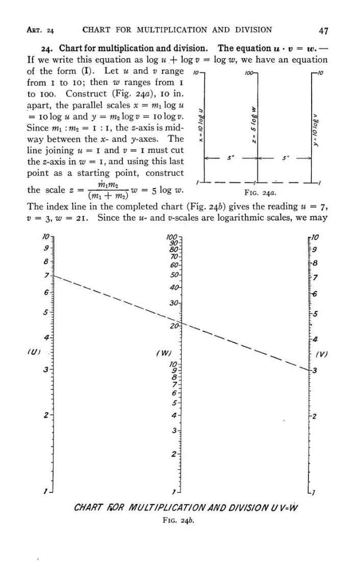
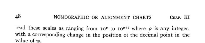
I merely flipped Lipka’s implementation by 90 degrees to better accomodate a landscape computer monitor.

As one last experiment, I decided to combine the adder and multiplier into a single interactive graphic. Each of the three scales now combines a linear scale on top and a logarithmic scale on bottom.

The values on the linear scale are 10 times the logarithms of the values on the logarithmic scale. The values on the logarithmic scale are 10 to the power of a tenth of the values on the linear scale.